
Chapter 7: Postsecondary Employment and Wage Outcomes: Controlling for Age, Gender, and Work Experience
Supplemental Material (Excel file)
The most difficult decision for many high school seniors is where to attend college. Students face several factors associated with college choice, including distance, financial costs, available financial aid, university characteristics, and economic climate. According to the National Center for Education Statistics (2011), the number of freshmen leaving their home state to attend college in another state has increased from 250,000 in 1992 to 392,000 in 2010. This presents many states with challenges regarding the loss of educated, skilled workers to other states. To assist in countering this trend, the U.S. has seen a recent shift in policy with the introduction of state merit-based student aid programs. Several reasons for this shift have been identified, including curtailing student out-migration with the hope of retraining skilled workers within a state (Dynarski, 2000).
Literature Review
The principal research areas when assessing student migration are out-migration and in-migration. In other words, the factors associated with students leaving their home state to attend an institution in another state (out-migration) and the factors associated with students coming into a state (in-migration). Tuckman (1970) analyzed data from each state and found that students are more likely to migrate out when tuition rates in a state are high even when origin-state financial aid is taken into account. Tuckman also suggested that as a state’s per capita income increased students were more likely to voluntarily migrate out due to the likely increase in financial assistance from parents. Mixon (1992) provided results similar to Tuckman, but included college quality as a variable. The results indicated that higher tuition rates in a state do lead to out-migration but that an increase in school selectivity (i.e., quality) decreased out-migration.
More recent studies suggest that other factors are influencing college choice above and beyond cost alone. The migration of students tends to be based on the price of tuition for both in-state and out-of-state schools, the overall quality of the institutions within a state, and geographic regions with greater employment outcomes after graduation. (Baryla & Dotterweich, 2001; Cooke & Boyle, 2011).
Students also face the added pressure of predicting their ability to obtain adequate employment after graduation. Hilmer (2002) analyzed data from the Baccalaureate and Beyond survey from the class of 1993 and compared the tuition rates of public and private four-year institutions both in and out-of-state to determine the effects of the type of college attended as an employment recruitment screening device. Hilmer found that students who attended private and public out-of-state institutions have a positive wage premium post-graduation over those students who graduated from similar in-state public institutions.
Funding for educational financial aid programs comes from federal, state, and local governments, and the colleges and institutions themselves. Currently, 16 states have adopted statewide merit-based student aid programs with Georgia’s HOPE scholarship introduced in 1993 as the first. Merit-based student aid programs have several proposed outcomes with the most important being educating and retaining highly skilled workers within a state (Dynarski, 2000) thus enhancing the workforce and improving economic development (and reducing brain drain). The number of states adopting merit-based aid programs is on the rise. Policymakers throughout states are looking at student migration and the loss of their well-educated individuals as a cause for concern. Several states that are considering merit-based aid programs have proposed that students who utilize these awards will be required to stay in the state for a certain number of years after graduation (Redden, 2007).
Many college students who move to an area to pursue postsecondary education will leave upon graduation. Students will often move back to their previous location or a new location entirely (Corcoran, Faggian, & Mccann, 2010; Franklin, 2003). However, some studies suggest that students will stay in the region where they attended college. Using follow-up surveys in 1994 and 1997 from the Baccalaureate and Beyond Longitudinal Study, Perry (2001) found that 84% of students attending school in their home state remained in the state for the next four years compared to 63% of students who migrated out and returned to their home state. In a similar study that tracked students for 10 to 15 years post-graduation, Groen (2004) found a more modest effect with a 10-percentage point increase for those students who attended a school in their home state who were still residing in their state compared to those who attended a school in another state.
While in school, students may develop a wide range of human capital and find ways to be productive in that region after graduation. Much research has focused on the migration of skilled, educated workers to geographic areas with more human capital. Berry and Glaeser (2005) and Waldorf (2009) suggest that areas already populated with well-educated individuals will continue to attract more well-educated people. The benefits of migrating to an area concentrated with well-educated individuals seem to stem from higher wages and a better suited labor market for skilled individuals in those areas (Chen & Rosenthal, 2008; Waldorf, 2009). Some net migration to certain areas may rest solely on the presence of an institution of higher learning. Winters (2011) analyzed a sample of 2,004 nonmetropolitan counties and the effect the presence of institutions of higher learning had on population growth and level of human capital. The results suggest that those areas considered college towns (e.g., areas where the age profile of in-migration is skewed to individuals ages 15 to 24) gained the highest net migration compared to nonmetropolitan areas where no higher education is available.
Methodology
Program evaluation is the systematic study that assesses the effectiveness of program outcomes and whether the program is operating as intended (Rossi, Freeman, & Lipsey, 1999). A survey of the literature reveals that the methods used for program evaluation have not been agreed upon by practitioners. Two main study designs have been proposed to evaluate the effectiveness of programs: experimental and non-experimental designs. In 2009, the Government Accountability Office (GAO) released a report outlining the benefits and drawbacks of both designs and gave recommendations on how to proceed with program evaluation in the future (GAO, 2009). This report can be found at http://www.gao.gov/products/GAO-10-30.
In social science research, experimental design is regarded as the only true way of inferring cause and effect. Experimental designs are those which are highly controlled and participants are randomly assigned to treatment and control groups, thus eliminating any confounding variables that interfere with the treatment outcome. Some programs are well suited to experimental design, especially when the evaluator has complete control over the program, when random assignment is ethical, and resources (e.g., time, funding) are available to conduct them.
Non-experimental designs encompass all other study designs that are not experimental in nature and include a wide range of options. LaLonde (1986) concluded that the use of non-experimental designs in program evaluation can allow biases and specification errors into the results and that experimental designs can control for these issues. However, several authors (Heckman & Smith, 1995; GAO, 2009) argue that using experimental designs in program evaluation also has its drawbacks and will eliminate the evaluation of some programs because of cost or ethical concerns.
Due to concerns regarding the use of non-experimental designs in program evaluation, research in this area has been conducted with various non-experimental methods (Rosenbaum & Rubin, 1983; Heckman & Hotz, 1989; Heckman & Smith, 1999). The research conducted has been successful in producing results similar to experimental designs using non-experimental designs. These authors conclude that there is not a single methodology that eliminates all biases or systematic errors and that the focus should be on the questions and outcomes the evaluator wants addressed in terms of program effectiveness. The authors also propose that using reliable and suitable data for both program participants and the control groups will produce the most reliable estimates of program effectiveness.
Results
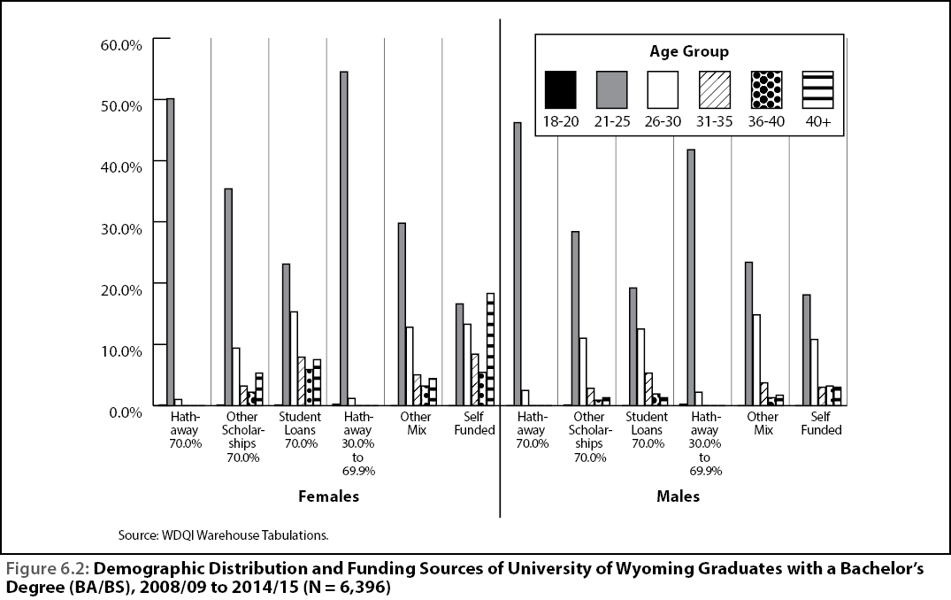
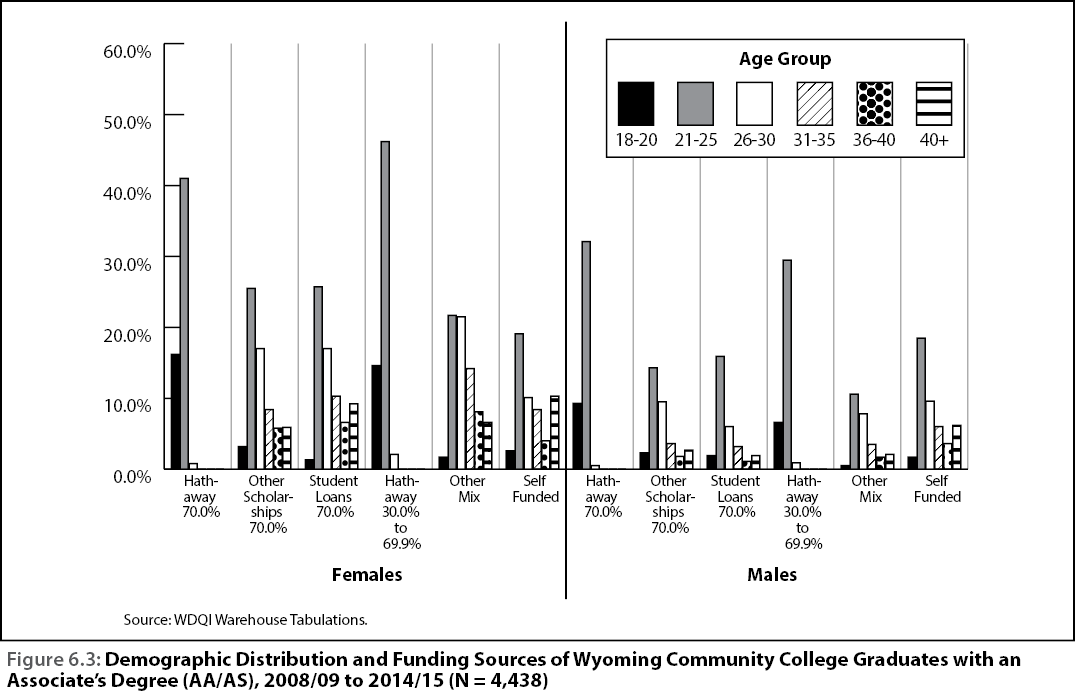
As shown in Chapter 6, the distribution of age and gender varied by student education and financing strategy (see Figures 6.2 and 6.3). In order to control for the differences in age, gender, work experience prior to graduation, and educational institution type, a stratified sample of those who received any financing source other than Hathaway Scholarship Program (HSP) was selected to match the HSP recipients. Individuals fell into the category of institutional type depending on whether or not their highest award came from a community college or UW. Graduates were excluded if they attended another postsecondary institution within two years of graduation.
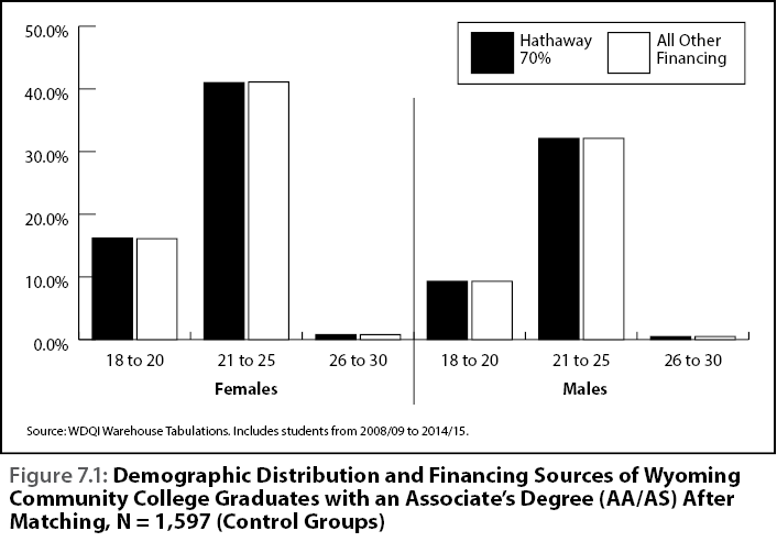
Individuals in the control group were selected based on age group and matched to similar individuals in the HSP group. HSP recipients included only those individuals who had 70% or more of their educational financing provided for by the HSP. After matching and as shown in Figures 7.1 and 7.2, the amount of variability in age and gender was significantly reduced by financing source compared to Figures 6.2 and 6.3 in Chapter 6. Those with an associate’s degree show more demographic variability than those with a bachelor’s degree. Employment and wages were analyzed for each of the eight quarters after graduation. For illustrative purposes, only the eighth quarter is discussed in this chapter.
Our primary finding is that the results are in a positive direction; however, after further analyses of the eight quarters following graduation, we found no significant differences for employment and wages for the HSP and comparison groups.
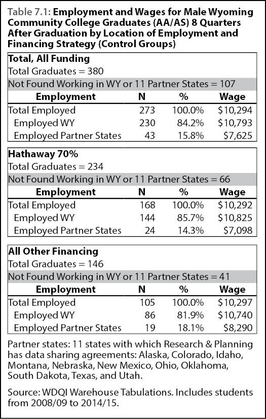
To illustrate interpretation of the results, the total numbers of potential college graduates are displayed by gender in Tables 7.1 to 7.4. After combining seven academic years, R&P accounted for the loss in employment and wages in later years due to lack of wage record administrative data beyond fourth quarter 2015 (2015Q4). For example, as shown in Table 7.1, there were a total of 380 male graduates with associate’s degrees, and 273 of those could be located either working in Wyoming or a partner state eight quarters after graduation. R&P could not account for the 107 graduates who did not appear in administrative datasets. These individuals are considered not found in the labor force for a variety of reasons, such as not working or working in a state with which R&P does not have a data sharing agreement.
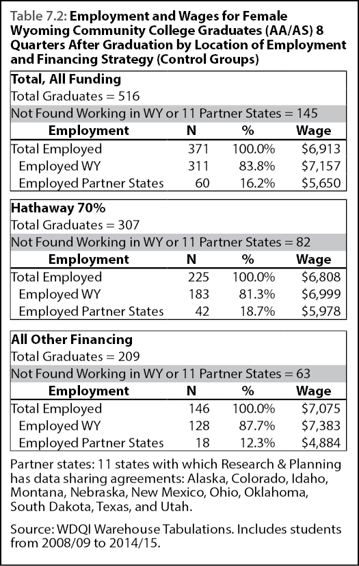
For those students who graduated with an associate’s degree, regardless of financing source, over 80% of both males (see Table 7.1) and females (see Table 7.2) were found working in Wyoming eight quarters after graduation. The largest percentage of students working in Wyoming eight quarters after graduation was females who earned an associate’s degree and received other sources of financing (87.7%; see Table 7.2).
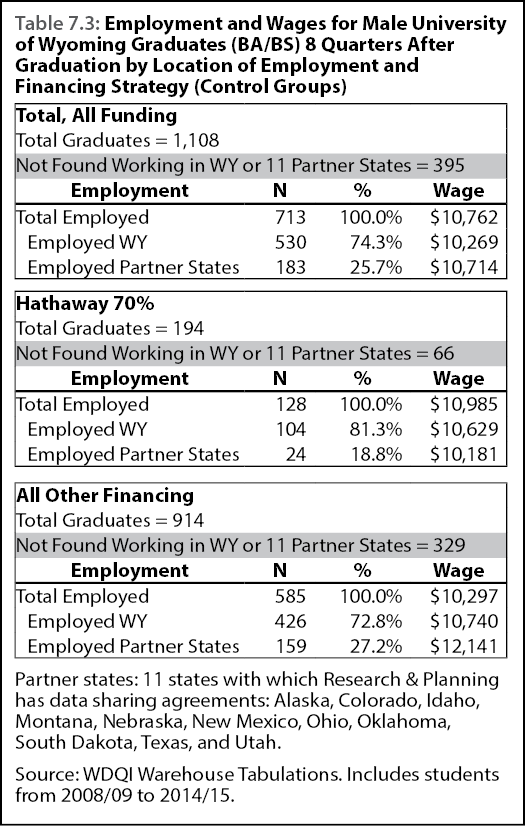
For those who graduated with a bachelor’s degree, overall the percentage working in Wyoming was lower compared to those who graduated with an associate’s degree. For example, 74.3% of males with a bachelor’s degree were still working in Wyoming eight quarters after graduation (see Table 7.3) compared to 84.2% of males with an associate’s degree (see Table 7.1).
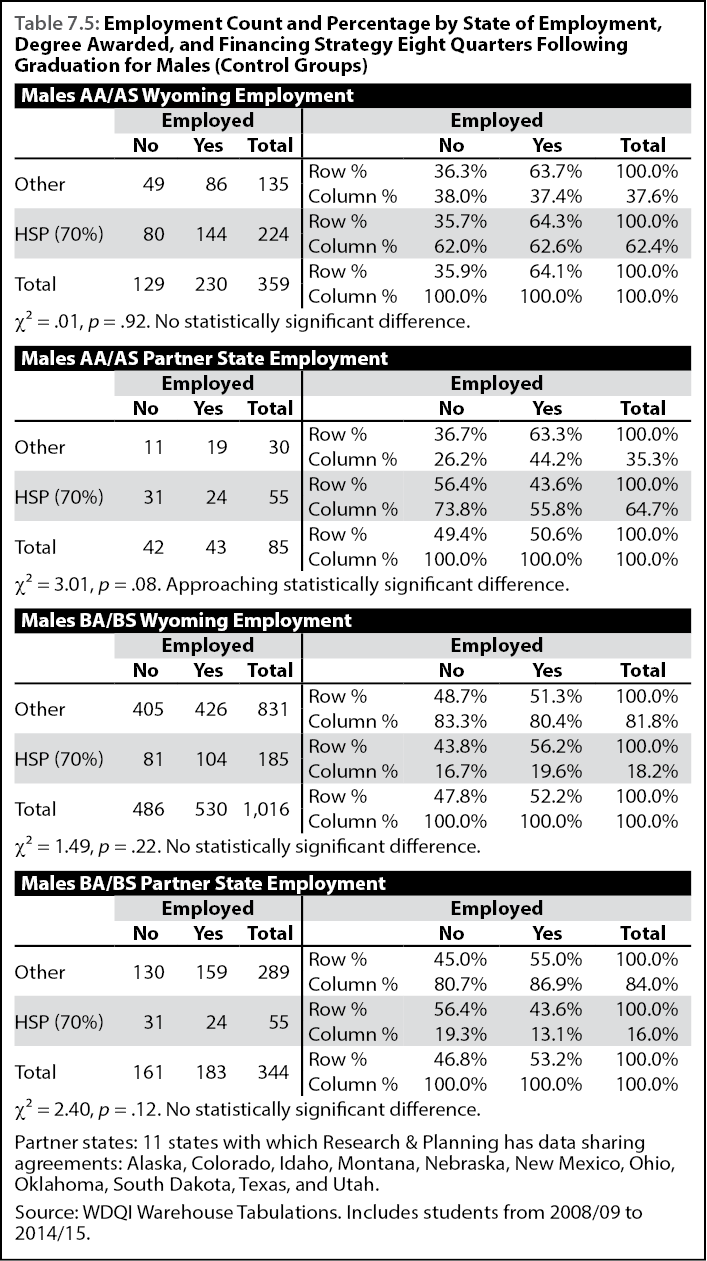
In order to test the differences in employment, R&P conducted multiple chi-square tests for independence on the percentage employed by financing source and state of employment. The chi-square for independence is a statistical test used to test the association between two categorical variables. The chi-square (χ²) does not tell the researcher how the variables are associated with each other, but only that there is an association between the variables. As seen in Table 7.5, a total of 359 males who graduated with an associate’s degree were analyzed. Of those who received 70% or more of their school financing through HSP, 144 (64.3%) were working in Wyoming while 80 (35.7%) were not found working in Wyoming. For those who received other financing, 86 (63.7%) were working in Wyoming and 49 (36.3%) were not found working in Wyoming. Comparing across financing sources, 37.4% of those who received other financing were working in Wyoming while 62.6% of those who received 70% or more of Hathaway financing were found working in Wyoming. However, the chi-square test failed to find a statistically significant difference between the two variables (χ² (2, N = 359) = .01, p =.92).
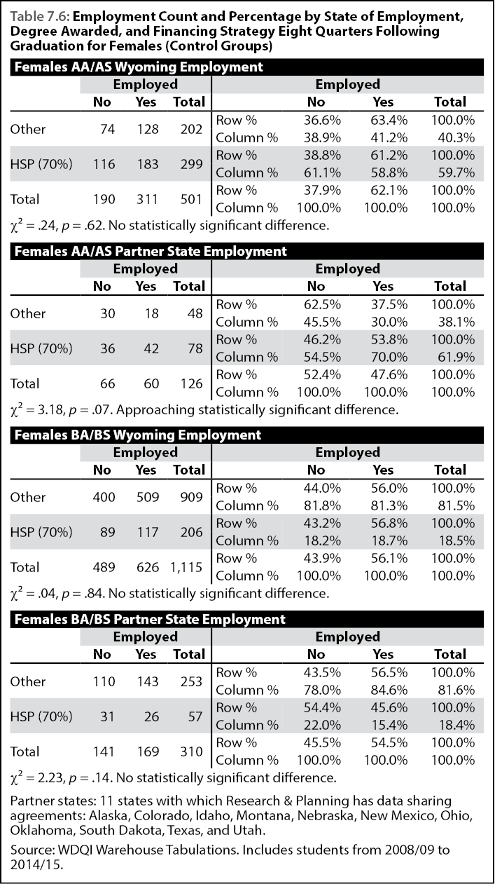
Females who graduated with an associate’s degree working in partner states approached significance (χ² (2, N = 126, p =.07). As seen in Table 7.6, 30.0% of those who received other financing were working in partner states eight quarters after graduation while 70.0% of those who received HSP financing were working in partner states.
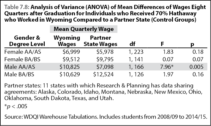
In terms of average wages, Tables 7.7 and 7.8 show the Analysis of Variance (ANOVA) results by gender, degree, financing source, and state of employment. Analysis of Variance was used to test mean differences between the populations due to the reduction in making a false positive (Type 1) error. An ANOVA is conceptually similar to a t-test for independent means but also tests for assumptions underlying the statistical test, such as homogeneity of variances between the groups compared.
Average quarterly wages were adjusted to 2015 levels using the Consumer Price Index (CPI). As seen in Table 7.7, wages were significantly higher for females who had 70% of their financing through HSP and graduated with a bachelor’s degree working in Wyoming eight quarters after graduation compared to those who received other financing. No other significant differences were observed between financing sources in the majority of the other seven quarters.
A goal of HSP is to retain a well-educated workforce. R&P conducted a comparison of wages in Wyoming to partner states. As seen in Table 7.8, males who received 70% of their financing through HSP and graduated with an associate’s degree earned significantly higher wages compared to those working in partner states. The opposite was found in the eighth quarter after graduation for males who graduated with a bachelor’s degree, although not statistically significant. The statistics reported in this chapter are available by clicking on this link to conduct independent analyses.
Conclusion
Hathaway impact has a positive direction for the retention of bachelor’s degree graduates, and female bachelor’s degree graduates who stay in Wyoming earn more than those who leave. However, the statistical test of bachelor’s degree graduate retention and earnings differences for females are equivocal and unconvincing.
This chapter examined the demographic distributions of the HSP recipients and those that received other financing for their education. After controlling for age, gender, and degree awarded, the employment distributions between the two financing sources examined were not found to have statistically significant differences in terms of employment across Wyoming or partner states. However, two effects were found in terms of wage differences between educational financing source and state of employment. Females who graduated with a bachelor’s degree with 70% of their financing coming from HSP and continued to work in Wyoming had a significantly higher mean quarterly wage eight quarters after graduation than those who received other financing. This difference may be due to the higher wages teachers and similar occupations receive in the state compared to surrounding states. For more information on teacher salaries, please see http://doe.state.wy.us/LMI/education_costs/2013/monitoring_2013.pdf.
Further, males with an associate’s degree financed through HSP earned significantly higher wages if employed in Wyoming compared to a partner state (see Table 7.8). These individuals may have graduated with technical degrees (e.g., welding) and began working in higher paying industries such as natural resources & mining. However, males who graduated with a bachelor’s degree earned higher wages if working in a partner state, although not statistically significant. One of the goals of HSP is to retain an educated workforce within Wyoming. Due to the limited number of quarters in the follow-up for some cohorts, R&P could not conduct a complete longitudinal analysis of employment and wages in the two to five years after graduation. Another limitation is the small N associated with some groups in the analysis. Caution should be used when comparing a small sample size with a larger sample size. Finally, the HSP has changed throughout its existence and different regulations and requirements were imposed on different cohorts which should be controlled for in future research. Further research should include an analysis of occupation and industry of employment after graduation. In addition, future research should focus on the interaction of college major and its influence on career trajectory and place of employment. For example, do those who receive a more technical education continue to reside in a state that has a demand for those specific jobs? Finally, as mentioned in the introduction, further examination of the effects of college major, labor market influences, social dynamics (e.g., family vs. career prioritization), and the ability for the Hathaway Scholarship to mediate these influences regarding employment outcomes. Student experience and employer hiring method relative to receiving a merit-based scholarship should be included in future analyses.
References
Barry, C.R., & Glaeser, E.L. (2005). The divergence of human capital levels across cities. Papers in Regional Science, 84, 407-444.
Baryla, E.A., & Dotterweich, D. (2001). Student migration: Do significant factors vary by region? Education Economics, 9, 269-280.
Chen, Y., & Rosenthal, S.S. (2008). Local amenities and life-cycle migration: Do people move for jobs or fun? Journal of Urban Economics, 64, 519-537.
Cooke, T.J., & Boyle, P. (2011). The migration of high school graduates to college. Educational Evaluation and Policy Analysis, 33, 202-213.
Corcoran, J., Faggian, A., & Mccann, P. (2010). Human capital in remote and rural Australia: The role of graduate migration. Growth and Change, 41, 192-220.
Dynarski, S. (2000). Hope for whom? Financial aid for the middle class and its impact on college attendance. National Tax Journal, 53, 629-661.
Franklin, R.S. (2003). Migration of the young, single and college educated: 1995 to 2000 (Census 2000 Special Reports, CENSR-12). Washington, DC: Government Printing Office.
Government Accountability Office (2009). Program evaluation: A variety of rigorous methods can help identify effective interventions (GA 1.13:GAP-10-30). Washington, DC: U.S. Government Printing Office.
Groen, J.A. (2004). The effect of college location on migration of college-educated labor. Journal of Econometrics, 121, 125-142.
Heckman, J.J., & Holz, V.J. (1989). Choosing among alternative methods for estimating the impact of social programs: The case for manpower training. Journal of American Statistical Association, 84, 862-874.
Heckman, J.J., & Smith, J.A. (1995). Assessing the case for social experiences. Journal of Economic Perspectives, 9, 85-110.
Heckman, J.J., & Smith, J.A. (1999). The pre-programme earnings dip and the determinants of participation in a social programme: Implication for simple program evaluation strategies. The Economic Journal, 109, 313-348.
Hilmer, M.J. (2002). Student migration and institution control as screening devices. Economic Letters, 76, 19-25.
LaLonde, R. (1986). Evaluating the econometric evaluations of training programs with experimental data. American Economic Review, 76, 604-620.
Mixon, F.G. (1992). Factors affecting college student migration across states. Internal Journal of Manpower, 13, 25-32.
National Center for Education Statistics (2011). The Digest of Education Statistics. Retrieved June 20, 2012, from http://nces.ed.gov/programs/digest/
Perry, K.K. (2001). Where college students live after they graduate. Washington, DC: National Center for Government Statistics. (ERIC Document Reproduction Service No. ED453739).
Redden, E. (2007, January 4). Tethering students to their states. Inside Higher Ed. Retrieved June 22, 2012, from http://www.insidehighered.com/news/2007/01/04/scholarships
Rosenbaum, P.R., & Rubin, D.B. (1983). The central role of the propensity score in observational studies for causal effects. Biometrika, 70, 41-55.
Rossi, P.H., Freeman, H.E., & Lipsey, M.W. (1999). Evaluation: A systematic approach (6th ed.). California: Sage.
Tuckman, H.P. (1970). Determinants of college student migration. Southern Economic Journal, 37, 184-189.
Waldorf, B.S. (2009). Is human capital accumulation a self-propelling process? Comparing educational attainment levels of movers and stayers. Annuals of Regional Science, 43, 323-344.
Winters, J. V. (2011). Human capital and population growth in nonmetropolitan U.S. counties: The importance of college student migration. Economic Development Quarterly, 25, 353-365.